Population splitting using Probplot
Input data are soil analyses from Daisy property, Montana (-80 mesh fraction, aqua-regia digestion, 0.5 gram aliquot). First 27 lines of input data file (ASCII) are as follows:
247 24 (Number of samples, number of variables)
“N” indicates
case or sample number type code is numeric; A would indicate it was
alphanumeric. “0” indicates length of alphanumeric case number (not applicable
in this case). “2”
defines the number of
numeric
fields immediately after the case number that are not to be analyzed. ”4”
defines the number of lines which contain the data from each case; and “6”
defines the number of variables on each of the 4 lines.
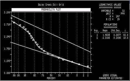
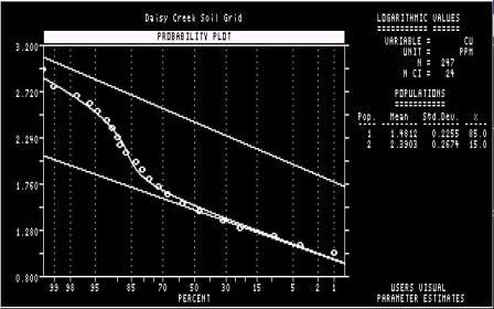
Daisy Creek Soil Grid
(Name of data
set. This will be reproduced on all graphical output)
ZN
PPM
AG PPM
NI
PPM
CO PPM
MN
PPM
FE
PCT
AS
PPM
SR
PPM
SB
PPM
SI PCT
V
PPM
CA PCT
P
PCT
LA PPM
CR
PPM
MG PCT
BA
PPM
TI
PCT
B
PPM
AL
PCT
NA
PCT
K PCT
(First
line of data follows)
7020 1550
1650 553.00 19.00
94.00 1.10 15.00
11.00
770.00 2.02
3.00 16.00 2.00
.06
31.00 .16
.13 12.00 10.00
.22
330.00 .11
8.00 2.45 .02
.13
|
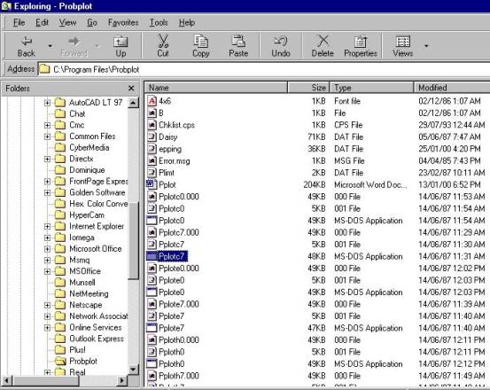
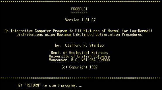
Step 1: Run PROBLOT
from Windows |
|
Introductory screen. No
action required (except hitting “RETURN”) |
|
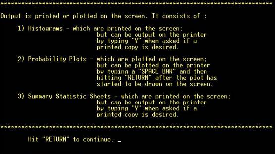
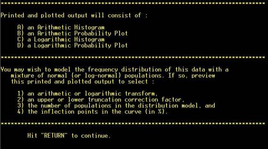
Output summary. No
action required (except hitting “RETURN”) |
|
No action required
(except hitting “RETURN”) |
|
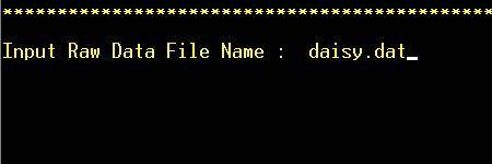
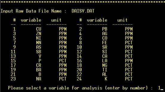
Step
2: Enter input data file name (for correct formatting of data in file,
see above) |
|
Step
3: Variable is selected by number |
|
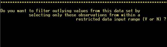
Step
4: Edit outliers from data, if desired. NOTE: Hot key (not necessary to
hit “RETURN”) |
|
No action required
(except hitting “RETURN”) |
|
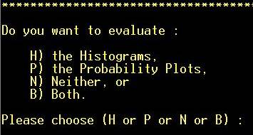
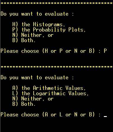
Step 5: Choose
evaluation method. “P” will be chosen in this case. NOTE: Hot key (not
necessary to hit “RETURN”) |
|
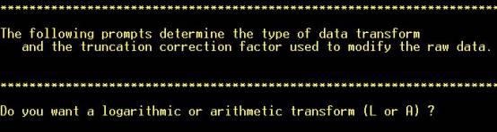
Step
6: Choose transformation method. “L” will be chosen in this case. NOTE:
Hot key (not necessary to hit “RETURN”) |
|
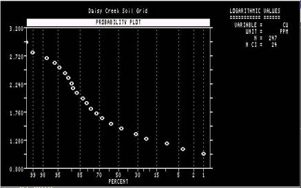
First cumulative frequency
plot. Advisable to print this out, or do a screen capture (PrtSc) and copy
into MS-Paint, so that it can be referred back to later. NOTE: X-axis scaled
in reverse order. The plot will disappear (and the program continue) if
“RETURN” is hit. |
|
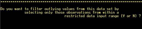
Step 7: Edit
outliers from data, if desired. NOTE: Hot key (not necessary to hit “RETURN”) |
|
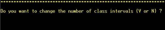
Step 8: Change number of class intervals, if desired. NOTE: Hot key (not necessary to hit “RETURN”). If “Y” is answered to either this or the preceding question, a new graph will be drawn |
|
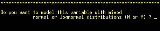
Step 9: The
important question being asked here is “Do you want
to model this variable with mixed distributions?”. Answering “N” will result in the program starting again with a new
variable. |
|
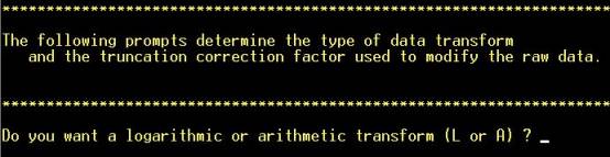
Step 10: Choose
whether to transform the data. Logarithmic transforms are commonly required
for trace-element geochemical data but ultimately this depends on the
frequency distribution of this element in this data set. NOTE: Hot key (not
necessary to hit “RETURN”). |
|
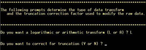
Answering “Yes” is appropriate
if a significant proportion of the analyses are “undetectable” (not in this
case). NOTE: Hot key (not necessary to hit “RETURN”). |
|
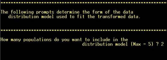
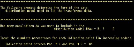
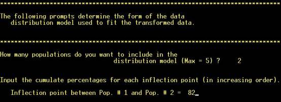
Step 11: Choose how
many subpopulations to model (inspect the cumulative frequency plot) |
|
Step 12: Read off an approximate
cutoff between the subpopulations from the X-axis of the cumulative frequency
plot |
|
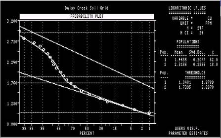
The samples falling
either side of the cutoff selected in Step 11 are assigned to two different
sub-populations. The curve represents the recombination of the two modelled
sub-populations, and the closeness of its correspondence to the observed
distribution represented by the points is an indication of how good the
cutoff estimate (of 85%) was. The program will continue if “RETURN” is hit. |
|
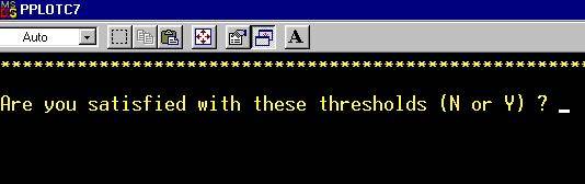
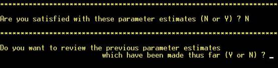
Step 13: A decision
is taken whether to seek a better cutoff. NOTE: Hot key (not necessary to hit
“RETURN”). |
|
Step 13: If “Y” is
hit, all previous estimates of the number of sub-populations, and the cutoffs
that separate them, will be listed on the screen. NOTE: Hot key (not necessary to hit “RETURN”). |
|
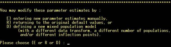
Step 14: To enter a
new estimate of the number of sub-populations, and the cutoffs that separate
them, hit “D”. If “E” is hit, the program will prompt the user for estimates
of the mean and standard deviation of the subpopulations. NOTE: Hot key (not
necessary to hit “RETURN”). |
|
Step 15: Step 10 is
repeated |
|
Step 16: Step 12 is
repeated, with a different cutoff between the two sub-populations |

|
Step 17: Once again,
the correspondence between the modelled subpopulations (curved line) and the
observed distribution (points) is evaluated. |
|
Step 18: As in Step 13, a decision is taken whether to seek
a better cutoff. NOTE: Hot key (not necessary to hit “RETURN”). In this case,
“Y” will be hit. NOTE: Hot key (not necessary to hit
“RETURN”). |
|
Step 19: If desired,
Probplot itself will seek an optimal split. This is not usually necessary if
there are only two subpopulations but more desirable if more than two are
identified. NOTE: Hot key (not necessary to hit “RETURN”). |
|
Step 20: The
“thresholds” in question refer to the mean plus two standard deviations of
each of the modelled populations represented by the straight, inclined lines.
They do not refer to the cutoffs, in analytical units, that separate the
subpopulations. NOTE: Hot key (not necessary to hit “RETURN”). |
|
Thresholds are
calculated. |
|
Step 21 (it is
necessary to execute the remaining 4 steps in order to exit from the
program). NOTE: Hot key (not necessary to hit “RETURN”). |
|
Step 22 NOTE: Hot key (not necessary to hit “RETURN”). |
|
Step 23 NOTE: Hot key (not necessary to hit “RETURN”). |