Selecting
an appropriate factor model by cross-validation, using Systat and Excel.
Input data are lake sediment analyses from Central Baffin Island (GSC Open File 3176), restricted to samples from lakes whose catchment basin is dominated by the Longstaff Bluff Formation (greywacke). Steps 1-2 and 7-12 are carried out in Excel; steps 3-6 are carried out in Systat.
|
Step 1 A column of random numbers between 0 and 1 is created using Excel’s intrinsic function. |
Step 2 The file is saved as tab-delimited text for input to Systat. |
|
Step 3 The file is loaded into Systat. |
Step 4 The data window appears. However, batch (macro) jobs cannot be run from it so it must be minimized. |

|
Step 5 The “Submit File” option is selected in the Output Organizer window. |
Step 6 A batch job entitled “bigfac.cmd” is selected. An abbreviated version follows |
Batch file for multiple factor-analysis
runs
This
file is loaded after the input file “bigfac.txt” has already been loaded,
although the load command can, if desired, be included in the list of batch
commands. Comments are included in bold. They should be removed or remmed out
before attempting to run the job in Systat.
The
best way to create a batch file from scratch is to do a test run interactively
and copy output in the Output Organizer (which monitors all the commands
entered) into a text editor where it can be altered and expanded. All batch
files should have the extension “.cmd”.
select rand
< 0.5
(this will select about
half the samples, on a random basis)
factor
(this starts the factor
analysis module in Systat)
save
"C:\My Documents\Short Course\f2a.syd" /loadings,single
(this instructs the
program to save the factor loadings in a Systat file, which will be converted
to Excel later in the batch job. The “2” refers to the number of factors that
will be extracted, and “A” refers to the random split)
model
As2_L,Ba,Br_L,Ce_L,Co1_L,Cr_S,Cs_S,Cu_L,Fe1_L,Hf_S,La_L,LOI_L,
Mn_L,Na,Ni_L,Pb_L,Rb_S,Sc_S,Sm,Ta_S,Tb_L,Th_L,U1_L,W_S,Yb_L,Zn_L,pH,
U_w_L
(this specifies the input
variables)
estimate
/pairwise,number=2,rotate,varimax
(this instructs the
program to extract 2 factors, perform a Varimax rotation. Loadings will be
saved according to earlier instruction)
factor
save
"C:\My Documents\Short Course\f3a.syd" /loadings,single
(the program is run
again, with loadings saved in a new file)
model
As2_L,Ba,Br_L,Ce_L,Co1_L,Cr_S,Cs_S,Cu_L,Fe1_L,Hf_S,La_L,LOI_L,
Mn_L,Na,Ni_L,Pb_L,Rb_S,Sc_S,Sm,Ta_S,Tb_L,Th_L,U1_L,W_S,Yb_L,Zn_L,pH,
U_w_L
estimate
/pairwise,number=3,rotate,varimax
(3 factors are extracted
this time)
(the process is run another 6 times, for
factor models 4 to 9 on the first random split)
…
select rand
> 0.5
(this will select the other random half of the samples)
factor
save
"C:\My Documents\Short Course\f2b.syd" /loadings,single
model
As2_L,Ba,Br_L,Ce_L,Co1_L,Cr_S,Cs_S,Cu_L,Fe1_L,Hf_S,La_L,LOI_L,
Mn_L,Na,Ni_L,Pb_L,Rb_S,Sc_S,Sm,Ta_S,Tb_L,Th_L,U1_L,W_S,Yb_L,Zn_L,pH,U_w_L
estimate
/pairwise,number=2,rotate,varimax
(the process is run
another 7 times, for factor models 3 to 9 on the second random split)
…
USE
"C:\My Documents\Short Course\f2a.syd"
EXPORT
"C:\My Documents\Short Course\f2a.xls" /TYPE=EXCEL
USE
"C:\My Documents\Short Course\f3a.syd"
EXPORT
"C:\My Documents\Short Course\f3a.xls" /TYPE=EXCEL
USE
"C:\My Documents\Short Course\f8b.syd"
EXPORT
"C:\My Documents\Short Course\f8b.xls" /TYPE=EXCEL
USE
"C:\My Documents\Short Course\f9b.syd"
EXPORT
"C:\My Documents\Short Course\f9b.xls" /TYPE=EXCEL
(all the Systat files are
converted to Excel)
|
Step 7 A new workbook is created, with worksheets for each factor model (in this case, 2 through 9) |
Step 8 The first of the output files from the factor analysis (f2a.xls) is loaded and the contents copied to the clipboard. |
|
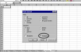
Step 9 The “Paste Special / Transpose Option is selected in the destination file. |
Step 10 Result |
|
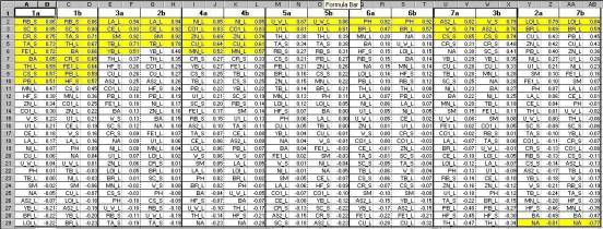
Step 11 The column containing variable names is copied and inserted before the loadings of the second factor; then the loadings for each factor are sorted in descending order and loadings greater than 0.5 are highlighted (0.5 is an arbitrary but useful cutoff figure). The loadings are labelled in the first row (1a and 2a). |
Step 12 The procedure is repeated with the contents of the file “f2b.xls”, with loadings for Factors 1b and 2b. Factors 1a and 1b, in which similar elements display strong loadings, are juxtaposed, as are factors 2a and 2b between which similarities are less strong. |
|
The optimal correspondence between the two random
splits was obtained with a 7-factor model |